Explaining Predictions: Boosted Trees Post-hoc Analysis (Xgboost)
Recap
We’ve covered various approaches in explaining model predictions globally. Today we will learn about another model specific post hoc analysis. We will learn to understand the workings of gradient boosting predictions.
Like past posts, the Clevaland heart dataset as well as tidymodels principle will be used. Refer to the first post of this series for more details.
Gradient Boosting
Besides random forest introduced in a past post, another tree-based ensemble model is gradient boosting. In gradient boosting, a shallow and weak tree is first trained and then the next tree is trained based on the errors of the first tree. The process continues with a new tree being sequentially added to the ensemble and the new successive tree improves on the errors of the ensemble of preceding trees. On the hand, random forest is an ensemble of deep independent trees.
#library
library(tidyverse)
library(tidymodels)
theme_set(theme_minimal())
#import
heart<-read_csv("https://archive.ics.uci.edu/ml/machine-learning-databases/heart-disease/processed.cleveland.data", col_names = F)
# Renaming var
colnames(heart)<- c("age", "sex", "rest_cp", "rest_bp",
"chol", "fast_bloodsugar","rest_ecg","ex_maxHR","ex_cp",
"ex_STdepression_dur", "ex_STpeak","coloured_vessels", "thalassemia","heart_disease")
#elaborating cat var
##simple ifelse conversion
heart<-heart %>% mutate(sex= ifelse(sex=="1", "male", "female"),fast_bloodsugar= ifelse(fast_bloodsugar=="1", ">120", "<120"), ex_cp=ifelse(ex_cp=="1", "yes", "no"),
heart_disease=ifelse(heart_disease=="0", "no", "yes")) #remember to leave it as numeric for DALEX
## complex ifelse conversion using `case_when`
heart<-heart %>% mutate(
rest_cp=case_when(rest_cp== "1" ~ "typical",rest_cp=="2" ~ "atypical", rest_cp== "3" ~ "non-CP pain",rest_cp== "4" ~ "asymptomatic"), rest_ecg=case_when(rest_ecg=="0" ~ "normal",rest_ecg=="1" ~ "ST-T abnorm",rest_ecg=="2" ~ "LV hyperthrophy"), ex_STpeak=case_when(ex_STpeak=="1" ~ "up/norm", ex_STpeak== "2" ~ "flat",ex_STpeak== "3" ~ "down"), thalassemia=case_when(thalassemia=="3.0" ~ "norm",
  thalassemia== "6.0" ~ "fixed", thalassemia== "7.0" ~ "reversable"))
# convert missing value "?" into NA
heart<-heart%>% mutate_if(is.character, funs(replace(., .=="?", NA)))
# convert char into factors
heart<-heart %>% mutate_if(is.character, as.factor)
#train/test set
set.seed(4595)
data_split <- initial_split(heart, prop=0.75, strata = "heart_disease")
heart_train <- training(data_split)
heart_test <- testing(data_split)
The gradient boosting package which we’ll use is xgboost. xgboost only accepts numeric values thus one-hot encoding is required for categorical variables. However, I was still able to train a xgboost model without one-hot encoding when I used the parsnip interface.
# create recipe object
heart_recipe<-recipe(heart_disease ~., data= heart_train) %>%
  step_knnimpute(all_predictors())
# process the traing set/ prepare recipe(non-cv)
heart_prep <-heart_recipe %>% prep(training = heart_train, retain = TRUE)
No tunning was done, the hyperparameters are default settings which were made explicit.
# boosted tree model
bt_model<-boost_tree(learn_rate=0.3, trees = 100, tree_depth= 6, min_n=1, sample_size=1, mode="classification") %>% set_engine("xgboost", verbose=2) %>%    fit(heart_disease ~ ., data = juice(heart_prep))
Feature Importance (global level)
The resulting gradient boosting model bt_model$fit represented as a parsnip object does not inherently contain feature importance unlike a random forest model represented as a parsnip object.
summary(bt_model$fit)## Length Class Mode
## handle 1 xgb.Booster.handle externalptr
## raw 66756 -none- raw
## niter 1 -none- numeric
## call 7 -none- call
## params 9 -none- list
## callbacks 1 -none- list
## feature_names 20 -none- character
## nfeatures 1 -none- numericWe can extract the important features from the boosted tree model with xgboost::xgb.importance. Although we did the pre-processing and modelling using tidymodels, we ended up using the original Xgboost package to explain the model. Perhaps, tidymodels could consider integrating prediction explanation for more models that they support in the future.
library(xgboost)
xgb.importance(model=bt_model$fit) %>% head()
## Feature Gain Cover Frequency
## 1: thalassemianorm 0.24124439 0.05772889 0.01966717
## 2: ex_STdepression_dur 0.17320374 0.15985018 0.15279879
## 3: ex_maxHR 0.10147873 0.12927719 0.13615734
## 4: age 0.07165646 0.09136876 0.12859304
## 5: chol 0.06522754 0.10151576 0.15431165
## 6: rest_bp 0.06149660 0.09178222 0.11497731Variable importance score
Feature importance are computed using three different importance scores.
- Gain: Gain is the relative contribution of the corresponding feature to the model calculated by taking each feature’s contribution for each tree in the model. A higher score suggests the feature is more important in the boosted tree’s prediction.
- Cover: Cover is the relative observations associated with a predictor. For example, feature X is used to determine the terminal node for 10 observations in tree A and 20 observations in tree B. The absolute observations associated with feature X is 30 and the relative observation is 30/sum of all absolute observation for all features.
- Frequency: Frequency refers to the relative frequency a variable occurs in the ensembled of trees. For instance, feature X occurs in 1 split in tree A and 2 splits in tree B. The absolute occurrence of feature X is 3 and the (relative) frequency is 3/sum of all absolute occurrence for all features.
Category variables especially those with minimal cardinality will have low frequency score as these variables are seldom used in each tree. Compared to continuous variables or to some extend category variables with high cardinality as they have are likely to have a larger range of values which increases the odds of occurring the model. Thus, the developers of xgboost discourage using frequency score unless you’re clear about your rationale for selecting frequency as the feature importance score. Rather, gain score is the most valuable score to determine variable importance. xgb.importance selects gain score as the fault measurement and arranges features according to the descending value of gain score resulting in the most important feature to be displayed at the top.
Plotting variable importance
xgbosst provides two options to plot variable importance.
- Using basic R graphics via
xgb.plot.importance - Using
ggplotinterface viaxgb.ggplot.importance. I’ll be using the latter.
The xgb.ggplot.importance uses the gain variable importance measurement by default to calculate variable importance. The default argument measure=NULL can be changed to use other variable importance measurements. However, based on the previous section, it will be wiser to leave the argument as the default.
The xgb.ggplot.importance graph also displays the cluster of variables that have similar variable importance scores. The xgb.ggplot.importance graph displays each variable’s gain score as a relative contribution to the overall model importance by default. The sum of all the gain scores will equal to 1.
xgb.importance(model=bt_model$fit) %>% xgb.ggplot.importance(
top_n=6, measure=NULL, rel_to_first = F) 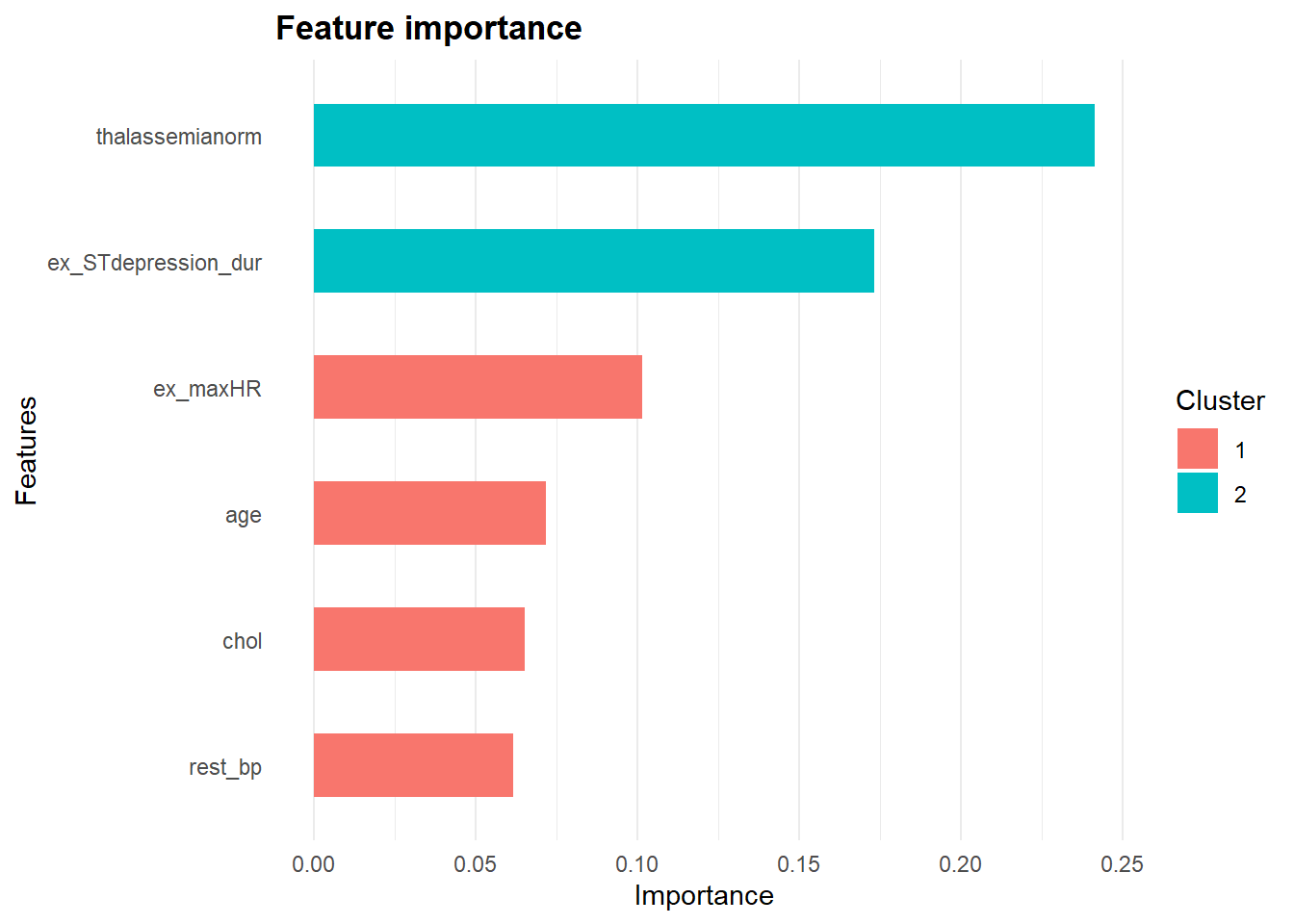
Alternatively, the gain scores can be presented as relative scores to the most important feature. In this case, the most importance feature will have a score of 1 and the gain scores of the other variables will be scaled to the gain score of the most important feature. This alternate demonstration of gain score can be achieved by changing the default argument rel_to_first=F to rel_to_first=T.
xgb.importance(model=bt_model$fit) %>% xgb.ggplot.importance(
top_n=6, measure=NULL, rel_to_first = T) 
Sum up
This is the last post of this series looking at explaining model predictions at a global level. We first started this series explaining predictions using white box models such as logistic regression and decision tree. Next, we did model specific post hoc evaluation on black box models. Specifically, for random forest and Xgboost.